Introducción a R: Tablas chulas y comandos estadísticos
2023

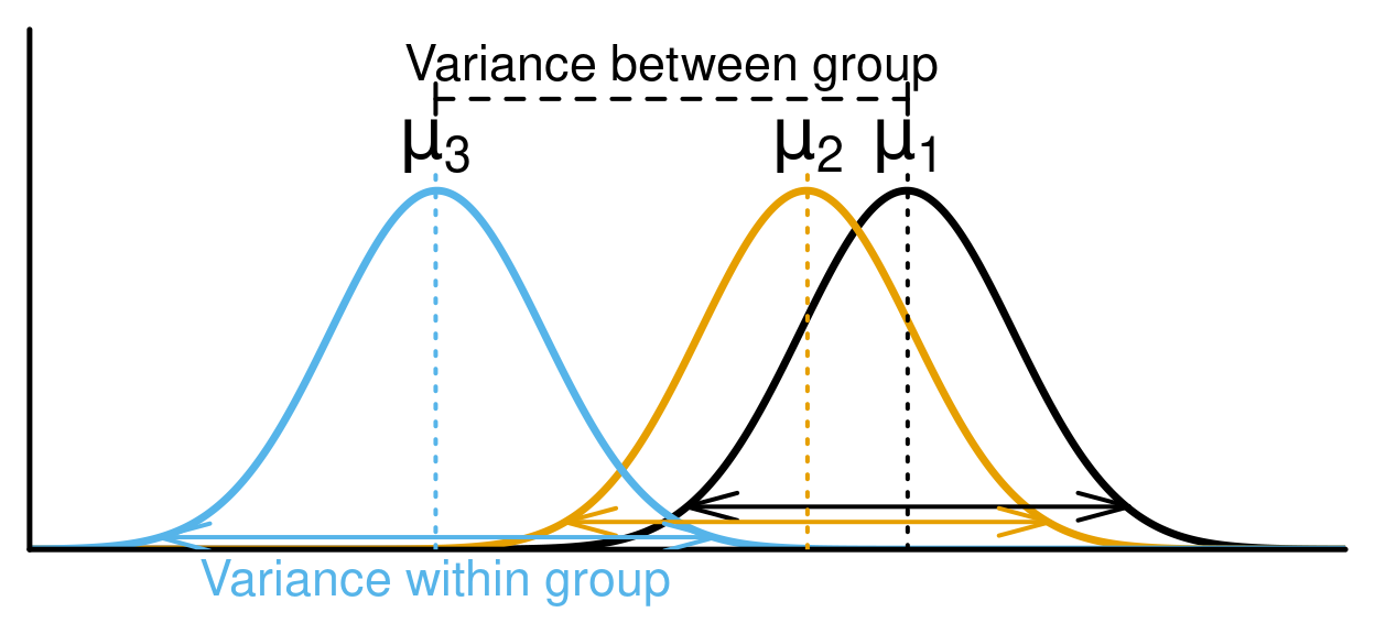
Imagen tomada de internet
Vamos a generar un conjunto de datos llamado “m_m” que contiene información sobre diferentes especies de mamíferos marinos. Queremos realizar diferentes tipos de tablas:
m_m <- data.frame(
Especie = c("Foca-freddy", "Delfín-flipper", "Ballena-migaloo", "León marino-aslan", "Orca-willy"),
Familia = c("Phocidae", "Delphinidae", "Balaenopteridae", "Otariidae", "Delphinidae"),
Longitud = c(2.5, 3.2, 18.7, 2.1, 9.5),
Peso = c(150, 200, 2500, 180, 400),
Habitat = c("Ártico", "Océano Atlántico", "Océano Pacífico", "Mar Mediterráneo", "Océano Atlántico")
)
head(m_m)-Especie: Nombre en la mayoría de los casos falso.
-Familia: Relacionada a la especie.
-Longitud: Longitud del animal en “metros”.
-Peso: Peso del animal en “kg”.
-Habitat: Zona donde habita el animal.

# Instalar el paquete knitr
#install.packages("knitr")
library(knitr)
# Crear una tabla con formato utilizando knitr
kable(m_m, format = "html", caption = "Mamíferos")| Especie | Familia | Longitud | Peso | Habitat |
|---|---|---|---|---|
| Foca-freddy | Phocidae | 2.5 | 150 | Ártico |
| Delfín-flipper | Delphinidae | 3.2 | 200 | Océano Atlántico |
| Ballena-migaloo | Balaenopteridae | 18.7 | 2500 | Océano Pacífico |
| León marino-aslan | Otariidae | 2.1 | 180 | Mar Mediterráneo |
| Orca-willy | Delphinidae | 9.5 | 400 | Océano Atlántico |


 Gráfica de los resultados


